Sparkify Project
Using Apache Spark’s Machine Learning Library (MLlib) to predict churn of customers of a popular music streaming service.
In this capstone project for the Udacity Data Scientist Nanodegree Program, I use Spark SQL and PySpark DataFrames to analyse a small subset of 125 MB of data from Sparkify’s user log file. Udacity provides the full dataset with 12GB on AWS S3. My code is scalable, and it can be used on a single machine or on a cluster platform like AWS EMR or IBM Cloud, to process and analyse vast amounts of data. I use a Jupyter notebook for the code. https://github.com/PeterSchuld/Sparkify
.

Project Overview
The imaginary start-up company Sparkify offers music streaming service to users in the USA. Many users stream their favourite songs to our service every day either using the free tier that places advertisements between the songs, or using the premium subscription model, where they stream the music for free but pay a monthly flat rate. Every time a user interacts with the service, such as playing songs, liking a song with a thumps-up, hearing an ad, or downgrading their service, it generates data. All this data contains key insides for keeping the users satisfied and helping Sparkify’s business thrive. Sparkify keeps a user log file with 18 fields for every user interaction (e.g., userId, name of song played, length of song played, name of artist). The company uses the distributed file system Apache Spark to store and analyse the user data. Apache Spark is an open-source distributed cluster-computing framework. Spark is a data processing engine developed to provide faster and easy-to-use analytics than Hadoop MapReduce.
Problem Statement
It is our task to classify users who are at risk to churn, either downgrade from premium to free tier or cancelling their service altogether. Users can upgrade, downgrade, or cancel their service at any time. If we can accurately classify vulnerable users before they leave (i.e., classifying “true positives”), Sparkify can offer them discounts and incentives, potentially saving the business millions in revenue. However, we should avoid falsely predicting churn for active users who would stay loyal anyway (i.e., avoid classifying “false positives”), because discounts and incentives are expensive.
Metrics
We want to develop a Supervised Machine Learning model for a binary classification task, prediction Churn = 1 or Churn=0 for every distinct UserID in the dataset. The data is provided in a json-file by Udacity.

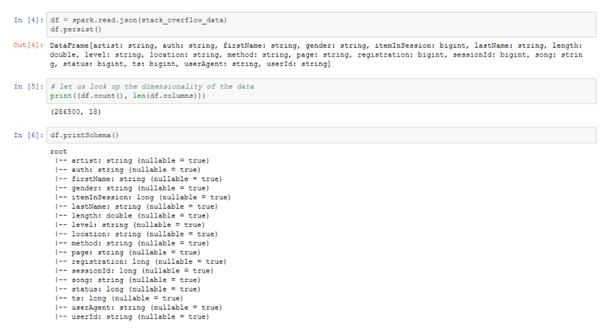
The small dataset (125 MB) consists of a dense matrix of 286,500 user records (i.e. rows) with 18 variables each (i.e. columns). During the data wrangling process, we clean the dataset and remove 8346 records with empty UserIDs. Those dropped records might belong to users who just tried the service without registration, and they would not help us predicting churn.
Next, we perform some preliminary data analysis on the cleaned PySpark DataFrame.
The user records were recorded in 4Q 2018.
Figure 1

There are 225 unique UserIDs in the dataset, of which 52 users cancelled the service at some point during 4Q 2018. Therefore, the dataset consists of 173 active users and 52 churned users. Most of the users in the dataset signed-up to the service in 2Q and 3Q 2018.
Figure 2

The ML model should correctly predict the label Churn=1 or Churn=0 for every UserID. We will measure the Accuracy of the predictions of the ML model. Accuracy is one metric for evaluating classification models. Informally, accuracy is the fraction of predictions our model got right. Formally, accuracy has the following definition:
Accuracy = Number of Correct Predictions / Total Number of Predictions
For binary classification, accuracy can also be calculated in terms of positives and negatives as follows:
Accuracy = ( TP + TN ) / ( TP + TN + FP + FN )
Where TP = True Positives, TN = True Negatives, FP = False Positives, and FN = False Negatives
Source:
https://developers.google.com/machine-learning/crash-course/classification/accuracy
However, Accuracy typically is not a good metric when the dataset classes are highly imbalanced. Therefore, we use a version of the F-score as a measure of the algorithm performance instead. Since the churned users are a small subset, we use the F1-score as the metric to optimize the ML model. We have 173 active users and only 52 churned users in the dataset (churn rate = 23 %).
The F1-score is optimal for imbalanced binary classification problems like churn prediction in the Sparkify dataset. The F1-score is suitable for imbalanced datasets because it is a harmonic mean of precision and recall.
Definition: F-score In statistical analysis of binary classification, the F-score or F-measure is a measure of a test's accuracy. It is calculated from the precision and recall of the test, where - the precision is the number of true positive results divided
  by  the number of all positive results, including those not
  identified correctly, and - the recall is the number of true positive results divided by
  the number of all samples that should have been identified as
  positive. - Precision is also known as positive predictive value, and recall
 is also known as sensitivity in diagnostic binary classification.

- The F1 score is the harmonic mean of the precision and recall. https://en.wikipedia.org/wiki/F-score
Our dataset is imbalanced with more active users than churned users, and we are most interested in correctly predicting TPs (i.e., correctly identified users who will churn) while keeping the number of FPs low (i.e. , loyal users anyway). However, we should keep the number of FNs low as well (i.e. , missed users who will churn). Precision is the share of the predicted positive cases which are correct:
precision = TP / (TP+FP)
Recall is the share of the actual positive cases which we predict correctly:
recall = TP / (TP+FN)
Therefore, using a mixture of precision and recall is suitable in our case. It ignores the high number of TNs (i.e., correctly classified active users who will stay loyal). The F1 score does this by calculating their harmonic mean:
F1 = 2 / (1/precision + 1/recall)
It reaches its optimum 1 only if precision and recall are both at 100%. And if one of them equals 0, then also F1 score has its worst value 0. If false positives and false negatives are not equally bad for the use case, Fᵦ is suggested, which is a generalization of F1 score.
Source: https://inside.getyourguide.com/blog/2020/9/30/what-makes-a-good-f1-score
Alternatively, the ROC-AUC is another classification metric suitable for imbalanced binary classification problems. However, I decided to use the F1-score as the most appropriate metric for this problem with a moderately imbalanced dataset (churn rate 23 percent).
https://developers.google.com/machine-learning/crash-course/classification/roc-and-auc
Exploratory Data Analysis (EDA)
Each record in the user log has 18 variables (i.e., rows). Most of them are self-explanatory, like userID, song, artist, length (of the song played), firstName (of the user). The variable ts (timestamp) shows the timing of the record in Unix-time, and the variable registration shows the timestamp when the user signed-up for the service.
Most of the records contain information about music played by the user. I use SQL queries to request data analytics from Spark, such as the most popular artists grouped by active and churned users, respectively.
Figure 3
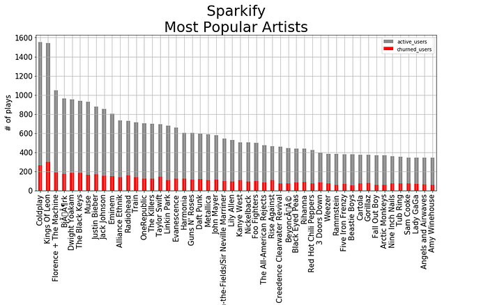
The SQL queries run on a temporary view. Creating additional variables that permanently stay as columns in the Spark DataFrame require PySpark commands instead.
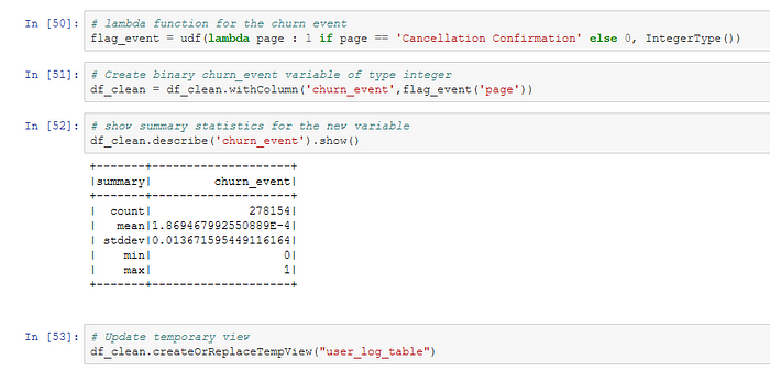
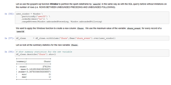
First, the label for the supervised ML model needs to be created by adding a new variable churn_event to the PySpark DataFrame. The PySpark syntax is similar to Python. However, in Pandas columnwise operations are recommended because they execute much faster. In PySpark we use element wise operations on each raw, using a lambda function in a user defined function to generate the new column. The lazy evaluation principle in Apache Spark requires the command .collect() or .show() to retrieve data from the PySpark DataFrame. Transformations are lazy in nature meaning when we call some operation in PySpark, it does not execute immediately. Furthermore, we need to update the temporary view if we want to run SQL queries on the new column. Second, I create the new variable Churn that indicates all the records of users who later cancel the service. We can use the SQL Windows function to get the maximum value of the variable churn_event for every userId.
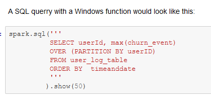
However, we want to add the column Churn to the PySpark DataFrame, and not only to the temporary view. Therefore, we use the PySpark Window function instead.
I use a similar approach with a PySpark Windows function to generate the new integer variable phase, which shows the number of times a user downgraded the service from premium to free-tier already. Like Churn, the variable phasehas one value for all the records of a user.
Other variables added to the PySpark DataFrame are usage_hours, no_of_items ,membership_days and session_count.
Data Visualization
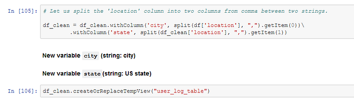
The variable location contains the state and city of a user. I create the new variables city and state, using PySpark.
We are most interested in location by state, and we aggregate the number of users accordingly, using a SQL query. The result is exported to Pandas with the .toPandas() command at the end of the SQL query.
Figure 4
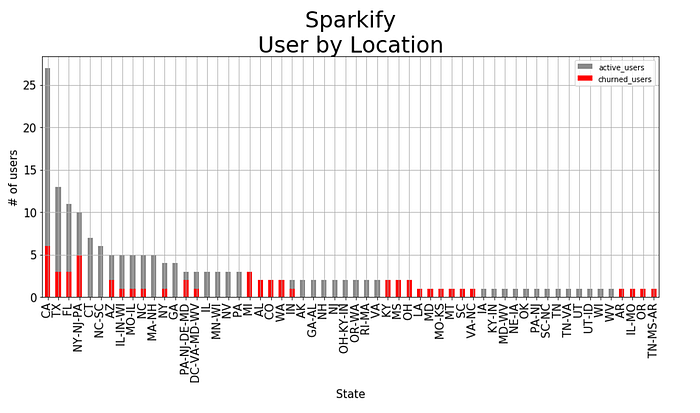
Most of Sparkify’s users are located in states with a large population. In the small dataset, Sparkify’s churn rate in CA, TX and FL is below the overall churn rate of 52/225 or 23 percent. However, Sparkify’s churn rate in several of the less populated states in the country is high.
Next, I use a SQL query with a temporary table (i.e. SQL WITH clause) to calculate averages for the categories of the page variable by user. The page variable shows the webpage on Sparkify’s service that the user visited. Furthermore, I have included averages for the new variables usage_hours, membership_days and session_count.
Figure 5
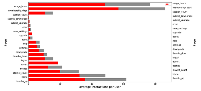
On average, active users show higher counts on all categories, but that is expected because churned users have spend less time on the service (i.e. , they have cancelled at some point). Therefore, we need to adjust for the average usage_hours and membership_days.
Figure 6
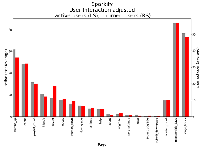
The visual adjustment reveals some differences between active users and churned users. Active users use more ‘thumbs-ups’, have more ‘friends’ and spend more time on the service, adjusted for menbership days. In contrast, churned users listen to more ‘adverts’, show more ‘thumbs-downs’ and have more ‘upgrades’.
Next, I added new variables for the timing of user interactions.
hour (string representing hour of the day),
day (string representing day of the week)
weekday. ( string representing day of the week)
Figure 7
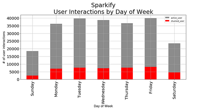
There is less traffic on weekends for both active users and churned users.
Next, I use user-agentsniffing to detect which type of devise the browser runs on. The variable user-agent contains the user-agent request header that lets servers and network peers identify the application, operating system, vendor, and/or version of the requesting user agent.
Figure 8
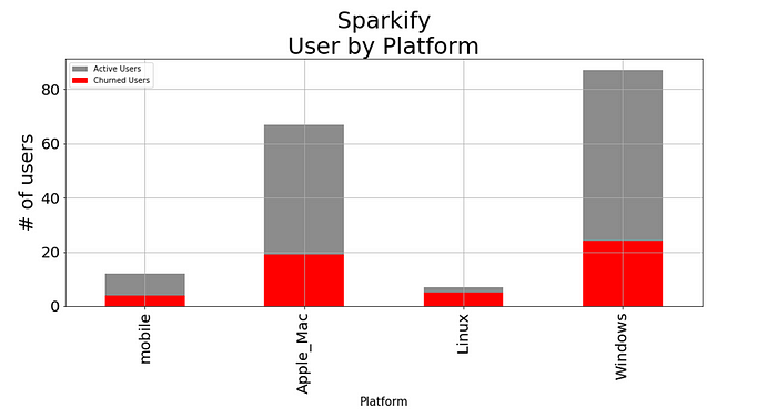
Linux users tend to churn the service more often. It is important that Sparkify’s customers are satisfied with the service on mobile devises as well, using mostly touch screen, because that is a customer segment with an attractive growth momentum.
We have reached the end of the Data Visualisation process. The PySpark DataFrame has been extended from the original 18 variables to 37 variables now.
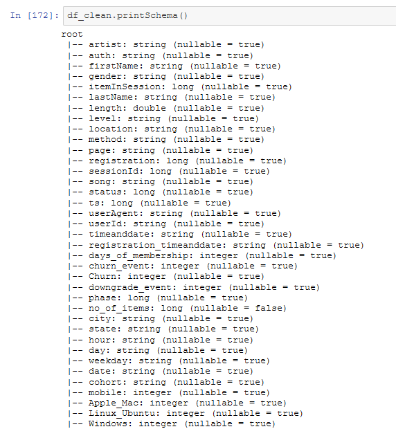
We need to make sure that all variables used in the ML model have a numerical data format. Hence, we need to change the column data types from string to integer for some variables.
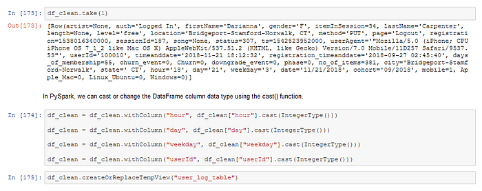
Feature Engineering
We write a SQL query to extract the necessary features from the PySpark DataFrame, and we create a new virtual table Feat_Engr with the result.
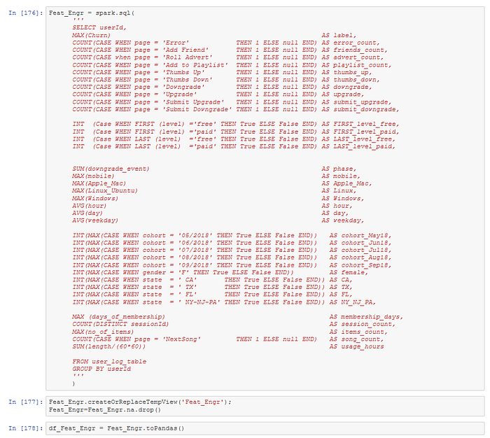
For better visibility, I upload the Feat_Engr table in Pandas as well. This step is not necessary if we want to keep the code scalable for big data application.
Let us look at the transpose of the Feat_Engr table, to see all the features as rows and users as columns.
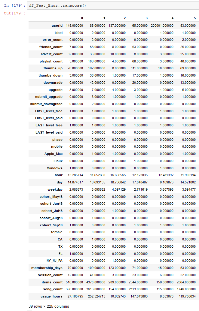
We get a table with one column for the label Churn, and 38 numerical features for each of the 225 users.
Modelling
Step 1. Train Test Split
As a first step we break our data set into 80% of training data and set aside 20%. Set random seed to 42.

Step 2. Create a Feature Vector
Create a vector from the combined columns of all the features.
VectorAssembler is a transformer that combines a given list of columns into a single vector column. It is useful for combining raw features and features generated by different feature transformers into a single feature vector, in order to train ML models like logistic regression and decision trees. VectorAssembler accepts the following input column types:
all numeric types, boolean type, and vector type. In each row, the values of the input columns will be concatenated into a vector in the specified order.https://spark.apache.org/docs/1.4.1/ml-features.html
Step 3. Normalize the Vectors
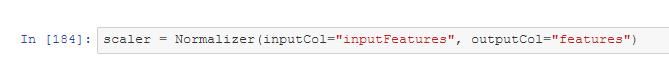
Normalizer is a Transformer which transforms a dataset of Vector rows, normalizing each Vector to have unit norm.
It takes parameter p, which specifies the p-norm used for normalization. (p=2 by default.) This normalization can help standardize your input data and improve the behavior of learning algorithms.
https://spark.apache.org/docs/1.4.1/ml-features.html
Step 4. Build Pipelines
Spark’s Machine Learning Library (MLlib) supports nine algorithms for Classification:
- Logistic regression
    Binomial logistic regression
    Multinomial logistic regression
- Decision tree classifier
- Random forest classifier
- Gradient-boosted tree classifier
- Multilayer perceptron classifier
- Linear Support Vector Machine
- One-vs-Rest classifier (a.k.a. One-vs-All)
- Naive Bayes
- Factorization machines classifier
I choose four of MLlib’s algorithms for our churn prediction task.
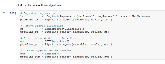
Logistic Regression Model
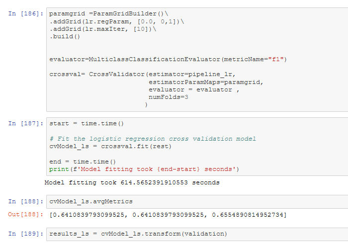
Let us tune the model. On the first 80% of the data let’s find the most accurate logistic regression model using 3-fold cross-validation with the following parameter grid:
- LogisticRegression regularization parameter: [0.0, 0.1]
- LogisticRegression max Iteration number: [10]
Refinement
Adding the parameter grid improves the performance of the Logistic Regression Model, but it extends the model fitting time. In the first run, I have used MLlib LogisticRegression without hyperparameter tuning using the following parameters:
lr = LogisticRegression(maxIter=10, regParam=0.0, elasticNetParam=0.0)Model fitting took 480.39185404777527 seconds
The time to fit the untuned Logistic Regression model is moderate, and the performance is encouraging (see below).
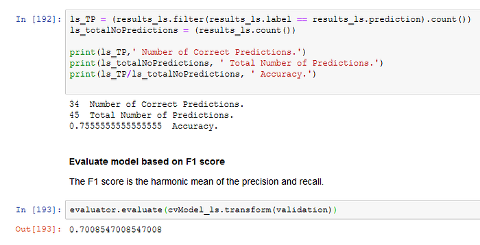
The F1-score of the untuned Logistic Regression model is 0.70 , and I decided to add the parameter grid for hyperparameter tuning.
The result of the tuned Logistic Regression Model:
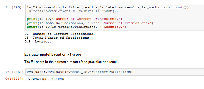
The F1-score of the tuned Logistic Regression Model is 0.73, which is an improvement compared to the untuned model. Furthermore, the time to fit the tuned Logistic Regression model is still moderate at 614 seconds on my local machine. Therefore, I decided to keep the tuned Logistic Regression Model.
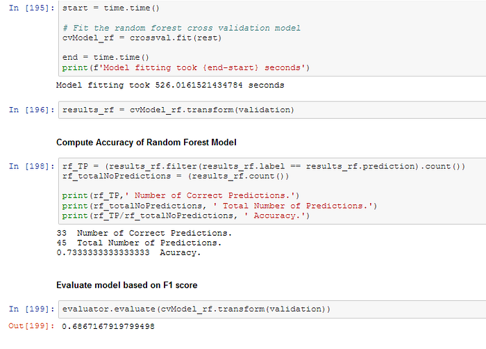
Random forest classifier
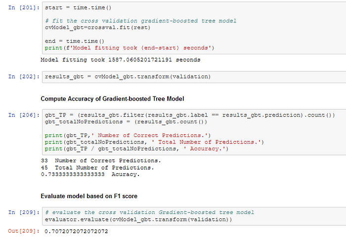
Gradient-boosted Tree classifier
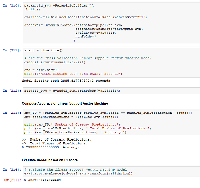
Linear Support Vector Machine
Results
The winning model for churn prediction is a tuned Logistic Regression Model that achieves a F1-score of 0.73 on the validation set.
for comparison:
F1-Score / Accuracy on the validation set (model fitting time)
- 0.73 / 0.80 Best Logistic Regression Model (615 seconds)
- [ 0.70 / 0.76 untuned Logistic Regression Model (480 seconds)]
- 0.69 / 0.73 Random Forest classifier (526 seconds)
- 0.71 / 0.73 Gradient-boosted Tree classifier (1587 seconds)
- 0.69 / 0.73 Linear Support Vector Machine (2886 seconds)
Model Evaluation and Validation
The Logistic Regression Model with hyperparameter tuning is the best solution for the churn prediction problem of the Sparkify user data. The model fitting time (615 seconds on my local machine) of the Logistic Regression Model including the parameter grid is much faster than the second best performing model, Gradient-boosted Tree classifier without tuning (1587 seconds). The F1-score of the Linear Support Vector Machine model is 0.69, and the time to fit the untuned model is excessive (2886 seconds).
The Random Forest classifier model has a F1-score of 0.69 , similar to the F1-score of 0.70 for the untuned Logistic Regression Model. However, the model fitting time for the untuned Random Forest classifier model (526 seconds) is significantly higher than the fitting time for the untuned Logistic Regression Model (480 seconds).
We want to maintain the scalability of the code, and model fitting time is critical for big data analytics. The Logistic Regression Model with hyperparameter tuning is the best solution for analysing large number of users in Sparkify’s 12 GB user log. This model has the best performance of all models tested, and the time requirement for model fitting is moderate. Logistic Regression is a robust model approach for the task, and it shows probabilities to churn for every user. Frequently running our model on Sparkify’s 12 GB user log, we could store those probabilities after each run, adding them to the user data. Going forward, we might be able to exploit some trends in the model predictions.
Reflection
In this project, we have uploaded a json-file with a small subset (125 MB) of Sparkify’s 12 GB user log into a PySpark DataFrame. After wrangling the data, we did preliminary data analysis on some of the 18 variables of the dataset. Next, we have performed Exploratory Data Analysis (EDA) on the cleaned PySpark DataFrame, adding new variables we have deemed useful for distinguishing churned users from active users. We have used PySpark commands to create new columns in the DataFrame, and Spark SQL queries to extract data from temporary views of the DataFrame. In Feature Engineering, we have created a virtual table, based on the result-set of an SQL query. The virtual table contains the label Churn, and 38 numerical features for each of the 225 users. In Modelling, we use the virtual table as input to create a Feature Vector required for Spark MLlib modelling. After Normalizing the vectors, we build pipelines for four different classification models. First, we have fitted an untuned Logistic Regression Model, which shows good results already. We use 3-fold cross-validation to better utilize the available dataset for training and test, leaving 20 percent of the data for validation. We choose the F1-score as the optimal metric for our binary classification problem, because the Sparkify dataset is imbalanced. Churned users are a small subset of all users in the dataset (churn rate 23 percent). We have decided to use hyperparameter tuning on the Logistic Regression Model to improve the performance further. The F1-score of the best tuned Logistic Regression Model is 0.73, with a moderate time requirement for model fitting. Second, we run a Random Forest classifier model on the data with cross-validation, using default settings for model tuning. While the time requirement for model fitting is moderate as well, the F1-score of 0.69 is well below the tuned Logistic Regression Model. Third, we run an untuned Gradient-boosted Tree classifier model with good performance (F1-score 0.71), but excessive time requirement for model fitting. Last, we run an untuned Linear Support Vector Machine with reasonable performance (F1-score 0.69), but with the longest time requirement for model fitting. Therefore, we have decided to choose the tuned Logistic Regression Model as the best solution for the Sparkify churn prediction problem.
I am very interested in Big Data analytics, using PySpark DataFrames and Spark SQL. Like most Data Analysts and Data Scientist I am familiar with Python, Pandas and SQL already, and the transition to Spark is relatively straightforward. During this project I have learned that is not necessary to deep dive into HDFS, MapReduce and Spark RDD to get your code running on Spark. However, debugging PySpark code can be challenging because some of the error messages can be confusing.
Improvement
The model performance could be enhanced by focussing more on the cohort analysis of the users. The analysis over the life cycle of users can help to get an understanding of the timing of a churn decision.
It would be interested trying different features with the large Sparkify dataset. I have not adjusted the features for time (e.g., song count/membership days), which might give the ML algorithm an unfair advantage. Furthermore, I would like to use features that capture the dynamic development of a decision to churn the service. For example, do users change their behaviour 2–4 weeks before churning?
Furthermore, the XGBoost and LightGBM models are promising supervised learning approaches to try next. Alternatively, since we’re creating multiple supervised learning models, we could try combining them all together into a custom ensemble model.
http://blog.kaggle.com/2016/12/27/a-kagglers-guide-to-model-stacking-in-practice/
https://www.kaggle.com/arthurtok/introduction-to-ensembling-stacking-in-python
Conclusion
Our PySpark’s MLlib Logistic Regression churn prediction model can help Sparkify to identify approx. 80 percent of the users who would churn. The company can use special promotions or other measures to prevent them from cancelling the service. The tuned Logistic Regression Model looks most suitable for the task, not least because it needs much less time to train than Gradient-boosted Tree classifier or Linear Support Vector Machine.